Combiners

Examples of a simple wilkison and branchline combiner.

import rfnetwork as rfn
import numpy as np
import matplotlib.pyplot as plt
from pathlib import Path

# set matplotlib style
plt.style.use(rfn.DEFAULT_STYLE)

# 50 ohm ms line on RO4350B substrate
msline50 = rfn.elements.MSLine(
    w=0.043,
    h=0.020,
    er=[3.758, 3.73, 3.722],
    loss=[0.03, 0.142, 0.266],
    frequency=[1e9, 5e9, 10e9]
)

# 70 ohm ms line on RO4350B substrate
msline70p7 = rfn.elements.MSLine(
    w=0.023,
    h=0.020,
    er=3.73,
    loss=0.152,
)

# 35 ohm ms line on RO4350B substrate
msline35= rfn.elements.MSLine(
    w=0.072,
    h=0.020,
    er=3.73,
    loss=0.1,
)

design_fhz = 5e9
# frequency vector for plots
frequency = np.arange(1e9, 9e9, 10e6)

## get quarter wavelength at the design frequency
len_qw_50 = msline50.get_wavelength(design_fhz).item() / 4
len_qw_70p7 = msline70p7.get_wavelength(design_fhz).item() / 4
len_qw_35 = msline35.get_wavelength(design_fhz).item() / 4

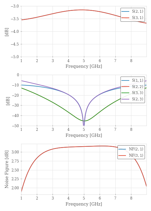
Wilkinson Combiner

class Wilkinson(rfn.Network):
    """
                 --- upper ----- port 2
                 |           |
       port 1 ----           r1
                 |           |
                 --- lower ----- port 3
    """
    # create line instances with specific length in inches
    upper = msline70p7(len_qw_70p7)
    lower = msline70p7(len_qw_70p7)

    r1 = rfn.elements.Resistor(100)

    p1 = msline50(.3)
    p2 = msline50(.3)
    p3 = msline50(.3)

    nodes = [
        ("P1", p1|1),
        ("P2", p2|2),
        ("P3", p3|2),
        (p1|2, upper|1, lower|1),
        (upper|2, r1|1, p2|1),
        (lower|2, r1|2, p3|1)
    ]

w = Wilkinson()

data = w.evaluate(frequency=frequency, noise=True)

# plot thru paths
fig, (ax1, ax2, ax3) = plt.subplots(3, 1, figsize=(5, 7))
w.plot(21, 31, fmt="db", frequency=frequency, axes=ax1)
ax1.set_ylim([-5, -3])

# plot isolation and return loss
w.plot(11, 22, 33, 23, fmt="db", frequency=frequency, axes=ax2)
ax2.set_ylim([-50, 0])

# plot passive noise figure
w.plot(21, 31, fmt="nf", frequency=frequency, axes=ax3)

fig.tight_layout()

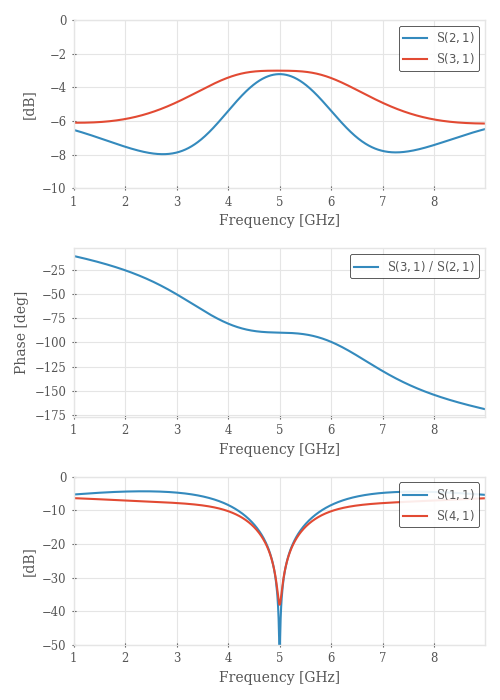
Branchline Coupler

class BranchCoupler(rfn.Network):
    """
      port 1 --------- top ---------- port 2
                 |                |
                left            right
                 |                |
      port 4 ----------btm ---------- port 3
    """

    top = msline35(len_qw_35)
    btm = msline35(len_qw_35)

    left = msline50(len_qw_50)
    right = msline50(len_qw_50)

    nodes = [
        # top left corner, port1
        (top|1, left|1, "P1"),
        # top right corner, port2
        (top|2, right|1, "P2"),
        # bottom corner, port 3
        (btm|2, right|2, "P3"),
        # bottom left, port 4
        (btm|1, left|2, "P4"),
    ]

b = BranchCoupler(passive=True)

fig, (ax1, ax2, ax3) = plt.subplots(3, 1, figsize=(5, 7))

# plot thru paths
b.plot(21, 31, fmt="db", frequency=frequency, axes=ax1)
ax1.set_ylim([-10, 0])

# plot phase angle
b.plot(31, ref=21, fmt="ang_unwrap", frequency=frequency, axes=ax2)

# plot isolation and return loss
b.plot(11, 41, fmt="db", frequency=frequency, axes=ax3)
ax3.set_ylim([-50, 0])

fig.tight_layout()

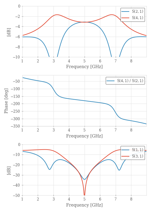
180 Hybrid Coupler

class Hybrid180(rfn.Network):
    """
    """

    s1 = msline70p7(len_qw_70p7)
    s2 = msline70p7(len_qw_70p7)
    s3 = msline70p7(len_qw_70p7)
    s4 = msline70p7(len_qw_70p7 * 3)

    nodes = [
        (s1|1, s4|2, "P1"), # Port A
        (s1|2, s2|1, "P2"), # A + B
        (s2|2, s3|1, "P3"), # Port B
        (s3|2, s4|1, "P4"), # A - B
    ]

b = Hybrid180(passive=True)

fig, (ax1, ax2, ax3) = plt.subplots(3, 1, figsize=(5, 7))

# plot thru paths
b.plot(21, 41, fmt="db", frequency=frequency, axes=ax1)
ax1.set_ylim([-10, 0])

# plot phase angle
b.plot(41, ref=21, fmt="ang_unwrap", frequency=frequency, axes=ax2)

# plot isolation and return loss
b.plot(11, 31, fmt="db", frequency=frequency, axes=ax3)
ax3.set_ylim([-50, 0])

fig.tight_layout()

Monopulse Comparator

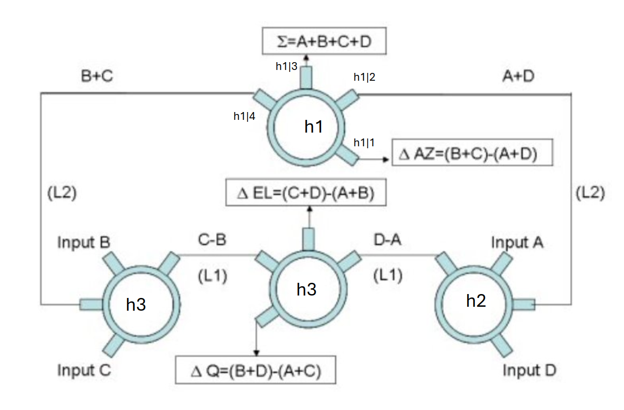
class MonopulseComparator(rfn.Network):
    """
    """

    h1 = Hybrid180()
    h2 = Hybrid180()
    h3 = Hybrid180()
    h4 = Hybrid180()

    line1 = msline50(0.4)
    line2 = msline50(0.4)
    line3 = msline50(0.2)
    line4 = msline50(0.2)

    r1 = rfn.elements.Resistor(50)

    nodes = [
        (h1|1, "P1"), # B + C - (A + D)
        (h1|3, "P2"), # SUM
        (h2|1, "P3"), # D
        (h2|3, "P4"), # A
        (h3|2, "P5"), # C + D - (A+B)
        (h4|2, "P6"), # B
        (h4|4, "P7"), # C
        (h3|4, r1|1),
        (r1|2, "GND"),
    ]

    cascades = [
        (h1|2, line1, h2|2),
        (h1|4, line2, h4|3),
        (h2|4, line3, h3|1),
        (h3|3, line4, h4|1)
    ]

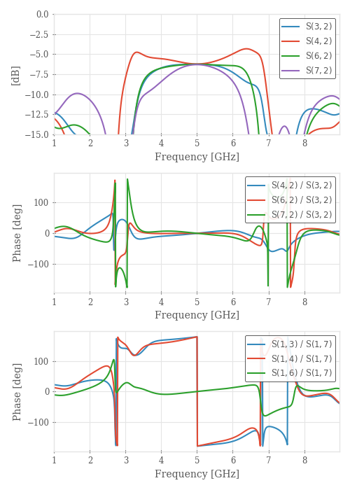
b = MonopulseComparator(passive=True)

b.evaluate()

fig, (ax1, ax2, ax3) = plt.subplots(3, 1, figsize=(5, 7))

# plot thru paths for sum port
b.plot(32, 42, 62, 72, fmt="db", frequency=frequency, axes=ax1)
ax1.set_ylim([-15, 0])

# plot phase of sum port
b.plot(42, 62, 72, ref=32, fmt="ang", frequency=frequency, axes=ax2)

# plot phase of difference port
b.plot(13, 14, 16, ref=17, fmt="ang", frequency=frequency, axes=ax3)

fig.tight_layout()
plt.show()