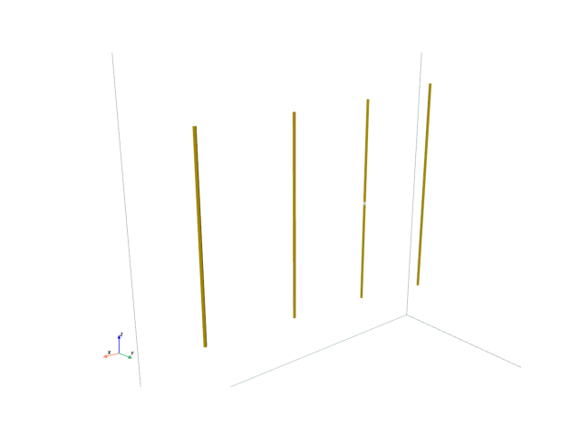
Yagi Antenna

Simulate UHF Yagi antenna and plot far-field gain.

from pathlib import Path
import numpy as np
import matplotlib.pyplot as plt
from rfnetwork import conv
import pyvista as pv

import rfnetwork as rfn
import mpl_markers as mplm

# set matplotlib style
plt.style.use(rfn.DEFAULT_STYLE)

try:
    dir_ = Path(__file__).parent
except:
    dir_ = Path().cwd()

User defined Parameters [inches]

f0 = 440e6
lam0 = rfn.const.c0_in / f0

# wire diameter
wire_d = 0.2
# gap between driver elements
gap = 0.2

# driver length
driver_len = 0.88 * (lam0 / 2)

# element lengths
reflector_len = lam0 * 0.49
director1_len = lam0 * 0.428
director2_len = lam0 * 0.416

# element spacing
sp = 0.195 * lam0

Build Yagi Model

def add_element(s: rfn.FDTD_Solver, x_loc: float, length: float, gap=0, resolution=4):
    """ Add a parasitic element to the yagi model at a x location with given length. """

    for z_center in (gap / 2 + (length / 4), -gap / 2 - (length / 4)):
        element = pv.Cylinder(
            center = (x_loc, 0, z_center),
            direction=(0, 0, 1),
            radius = wire_d / 2,
            height = length / 2,
            resolution=resolution
        )
        s.add_conductor(element, style=dict(color="gold"))

# solve box
sbox = pv.Cube(center=(sp/2, 0, 0), x_length=lam0 * 1.1, y_length=lam0 / 2, z_length=lam0)

# create model and add elements
s = rfn.FDTD_Solver(sbox)
add_element(s, x_loc=0, length=driver_len, gap=gap)
add_element(s, x_loc=-sp, length=reflector_len)
add_element(s, x_loc=sp, length=director1_len)
add_element(s, x_loc=2.1*sp, length=director2_len)

# add port in driver element
port1_face = pv.Rectangle([
    (0, -wire_d/2, gap/2),
    (0, wire_d/2, gap/2),
    (0, wire_d/2, -gap/2)
])
s.add_lumped_port(1, port1_face, "z-")

# PML boundaries are required on all sides to add a far-field monitor
s.assign_PML_boundaries("x-", "x+", "y-", "y+", "z+", "z-", n_pml=5)
s.generate_mesh(d_max = 0.5, d_min=0.1)

# setup far-field monitor
s.add_farfield_monitor(frequency=f0)

# show model rendering
cpos = pv.CameraPosition(
    position=(25, 25, 10),
    focal_point=(5, 0, 0),
    viewup=(0, 0.0, 1.0),
)

fig, ax = plt.subplots()
plotter = s.render(show_mesh=False, show_rulers=False, axes=ax, camera_position=cpos)

Setup Excitation and Solve

vsrc = s.gaussian_source(width=800e-12, t0=500e-12, t_len=30e-9)

s.assign_excitation(vsrc, 1)
s.solve(n_threads=4)

Running solver with 247.8k cells, and 6696 time steps...

Done in 21.552s

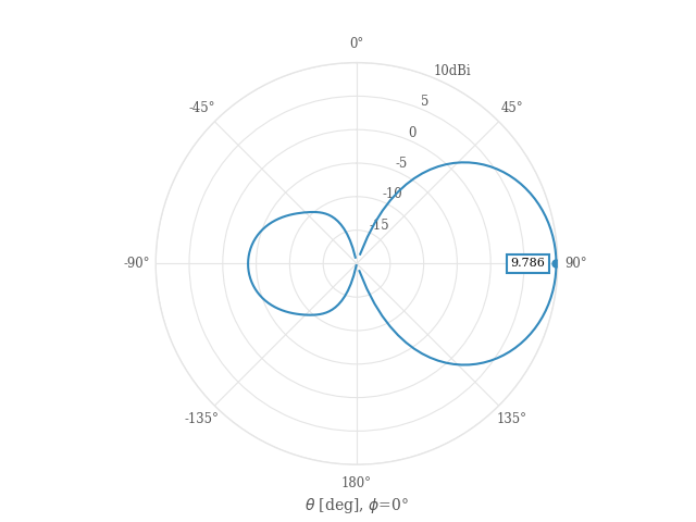
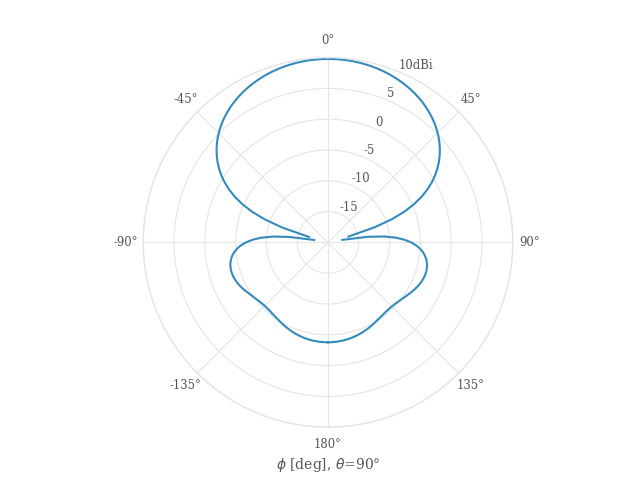
Principal Plane Cut at phi=0°

This plot shows realized gain

phi_cut = rfn.conv.db10_lin(
    s.get_farfield_gain(phi=np.arange(-180, 182, 2), theta=90).sel(polarization="thetapol")
)

theta_cut = rfn.conv.db10_lin(
    s.get_farfield_gain(theta=np.arange(-180, 181, 2), phi=0).sel(polarization="thetapol")
)

fig1, ax1 = plt.subplots(subplot_kw=dict(projection="polar"))
fig2, ax2 = plt.subplots(subplot_kw=dict(projection="polar"))

theta_rad = np.deg2rad(theta_cut.coords["theta"])
phi_rad = np.deg2rad(phi_cut.coords["phi"])

ax1.plot(theta_rad, theta_cut.squeeze())
ax2.plot(phi_rad, phi_cut.squeeze())

for ax in (ax1, ax2):
    ax.set_theta_zero_location('N')
    ax.set_theta_direction(-1)
    ax.set_ylim([-20, 10])
    ax.set_yticks(np.arange(-20, 15, 5))
    ax.set_yticklabels(["", "-15", "-10", "-5", "0", "5", "10dBi"])

    # Set theta labels
    ax.set_xticks(np.linspace(0, 2 * np.pi, 8, endpoint=False))
    labels = [f"{d}°" for d in [0, 45, 90, 135, 180, -135, -90, -45]]
    ax.set_xticklabels(labels)

ax1.set_xlabel(r"$\theta$ [deg], $\phi$=0°")
ax2.set_xlabel(r"$\phi$ [deg], $\theta$=90°")
mplm.line_marker(x=np.pi/2, axes=ax1, xline=False)

fig.tight_layout()

• 
• 

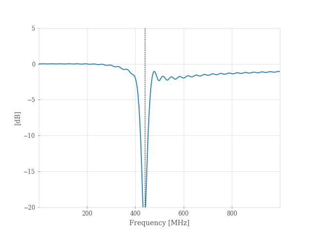
Plot S11

frequency: np.ndarray = np.arange(1e6, 1e9, 1e6)
sdata = s.get_sparameters(frequency, downsample=False)
S11 = sdata[:, 0]

fig, ax = plt.subplots()
ax.plot(frequency / 1e6, conv.db20_lin(S11))
ax.set_ylim([-20, 5])
ax.set_xlabel("Frequency [MHz]")
ax.set_ylabel("[dB]")

mplm.line_marker(x=f0 / 1e6, ylabel=False)
plt.show()