Note
Go to the end to download the full example code.
Combline Filter
Simulate a bandpass interdigital filter implemented with stripline resonators.
This follows the design process outlined in section 10.06 of [1], using a feed tap instead of a impedance transformer. The two extra coupled lines in the reference design were used to transform the impedance at the ends of the reactive elements. This leads to very small line spacings if attempted with thin stripline. The feed tap approach drops the outer resonators and avoids the issue of small spacings, but does require some manual tuning.
[1] G. L. Matthaei, Microwave Filters, Impedance-Matching Networks, and Coupling Structures, 1980
from pathlib import Path
import numpy as np
import matplotlib.pyplot as plt
import pyvista as pv

from np_struct import ldarray
import rfnetwork as rfn

# set matplotlib style
plt.style.use(rfn.DEFAULT_STYLE)

try:
    dir_ = Path(__file__).parent
except:
    dir_ = Path().cwd()
Design Parameters
er = 3.66  # dielectric constant
b = 0.06  # substrate height, inches

# cutoff frequencies
f1 = 1.1e9
f2 = 1.6e9

# 50 ohm trace width
w50 = 0.035

# tap location of feed, distance from the shorted end of the first resonator.
tap_loc = 0.31
# length of feed
feed_len = 0.12
# size of vias used to short ends of the resonators
via_size = 0.02

# filter order (must be odd)
N = 5

# quarter wave resonator length, inches
resonator_length = rfn.const.c0_in / (np.sqrt(f1 * f2) * np.sqrt(er) * 4)

# compensation for fringing fields on open-circuited ends of resonators. The design reference used 0.216", but the
# side walls were closer.
line_foreshortening = 0.095

# the tap on the outer resonators loads them and requires the length to be manually tuned. I couldn't find a good
# reference on this. The inner resonators are slightly adjusted to optimize the filter response.
resonator_length_tune = np.array([0.065, 0.01, -0.005, 0.01, 0.065])

# filter prototype values
g = rfn.utils.chebyshev_prototype(N, ripple=0.25)

# get even mode capacitance for each line (Ck), and the inter-line capacitance Cmk. Cmk is not the same thing as
# the odd mode capacitance. h is a free parameter used to adjust the line widths.
Ck, Cmk = rfn.utils.combline_sections_nb(g, f1, f2, er=er, h=0.25)

# The filter synthesis equations in the reference were intended for rectangular bars. When used for stripline in a
# narrow dielectric, they seem to overestimate the required inter-line capacitance. I've checked that the even/odd
# mode impedance used to derive the spacing is correct, so I suspect the reference equations more than the equations
# used to derive the spacing from the inter-line capacitance.
Cmk = (Cmk * 0.85)

# derive the line width and spacing from the line capacitances
wk, sk = rfn.utils.synthesize_combline_stripline(Ck, Cmk, b, er)

# we are using a tap instead of the outer lines to transform the impedance, so drop the outer resonators.
wk = wk[1:-1]
sk = sk[1:-1]

print("wk", wk)
print("sk", sk)
wk [0.0182248  0.0201692  0.02045788 0.0201692  0.0182248 ]
sk [0.01536218 0.01925833 0.01925833 0.01536218]
Build Filter Model
# upper location where lines are shorted to the side wall in the reference design, lower short location is 0
ymax = resonator_length
# lower and upper points of open-circuited ends of the nominal resonator lines
y0 = line_foreshortening
y1 = ymax - line_foreshortening
# x location of left side of first resonator
x_start = 0.1 + feed_len
# x location of right side of last resonator
x_end = x_start + np.sum(wk) + np.sum(sk)
# extent of solve box along x axis
xmax = x_end + feed_len + 0.1
# the reference design used a side wall to short the resonators, we are using vias, so add a bit of a buffer between
# the resonator ends and the side wall.
sbox_len = ymax + 0.15
# initialize model
substrate = pv.Cube(center=(xmax/2, sbox_len/2 - (0.15 / 2), 0), x_length=xmax, y_length=sbox_len, z_length=b)
sbox = pv.Cube(center=(xmax/2, sbox_len/2 - (0.15 / 2), 0), x_length=xmax, y_length=sbox_len, z_length=b)
s = rfn.FDTD_Solver(sbox)
s.add_dielectric(substrate, er=er, loss_tan=0.003, f0=np.sqrt(f1 * f2), style=dict(opacity=0.0))
# create resonators with the shorting vias
x0_i = x_start
# save lines for edge correction
lines = []
for i in range(N):
# bottom of first line (0, even) is shorted, top of second line (1, odd) is shorted.
# top of first line (0, even) is open, bottom of second line (1, odd) is open
if i % 2 == 0:
y0_i = 0
# adjust for tuned length on the open-circuited end of the line
y1_i = y1 + resonator_length_tune[i]
else:
y0_i = y0 + resonator_length_tune[i]
y1_i = ymax
# create resonator line
x1_i = x0_i + wk[i]
line = pv.Rectangle([(x0_i, y0_i, 0), (x1_i, y0_i, 0), (x1_i, y1_i, 0)])
s.add_conductor(line, style=dict(color="gold"))
# add shorting vias, bottom of resonator if even, top if odd
via_y = (y0_i - via_size, y0_i) if i % 2 == 0 else (y1_i, y1_i + via_size)
via = pv.Box((x0_i, x1_i, *via_y, -b / 2, b / 2))
s.add_conductor(via, style=dict(color="gold", opacity=0.6))
# increment edge for next resonator
if i < (N - 1):
x0_i = (x1_i + sk[i])
lines.append(line)
# add feed taps and lumped ports
feed_1 = pv.Rectangle([
(x_start - feed_len, tap_loc - w50 / 2, 0),
(x_start - feed_len, tap_loc + w50/ 2, 0),
(x_start, tap_loc + w50 / 2, 0),
])
feed_2 = pv.Rectangle([
(x_end + feed_len, tap_loc - w50 / 2, 0),
(x_end + feed_len, tap_loc + w50 / 2, 0),
(x_end, tap_loc + w50 / 2, 0),
])
s.add_conductor(feed_1, style=dict(color="gold"))
s.add_conductor(feed_2, style=dict(color="gold"))
port1_face = pv.Rectangle([
(x_start - feed_len, tap_loc - w50 / 2, -b/2),
(x_start - feed_len, tap_loc + w50 / 2, -b/2),
(x_start - feed_len, tap_loc + w50 / 2, b/2),
])
port2_face = pv.Rectangle([
(x_end + feed_len, tap_loc - w50 / 2, -b/2),
(x_end + feed_len, tap_loc + w50 / 2, -b/2),
(x_end + feed_len, tap_loc + w50 / 2, b/2),
])
# integration lines for the ports extend from the bottom of the dielectric to the middle where the lines are.
integration_line1 = pv.Line((x_start - feed_len, tap_loc, -b / 2), (x_start - feed_len, tap_loc, 0))
integration_line2 = pv.Line((x_end + feed_len, tap_loc, -b/ 2), (x_end + feed_len, tap_loc, 0))
s.add_lumped_port(1, port1_face, integration_line=integration_line1)
s.add_lumped_port(2, port2_face, integration_line=integration_line2)
cpos = pv.CameraPosition(
position=(xmax/2 + 0.5, -0.5, 1.1),
focal_point=(xmax/2, 0.4, 0),
viewup=(0, 0.0, 1.0),
)
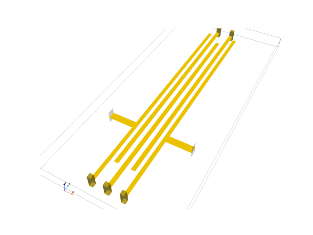
fig, ax = plt.subplots()
# render the model before generating the mesh to check for any obvious errors
s.render(show_mesh=False, show_rulers=False, axes=ax, camera_position=cpos)
# mesh with a minimum grid cell size of 5mils. This is fairly coarse for line spacings of 15mils and
# requires edge correction
s.generate_mesh(d_max = 0.02, d_min = 0.005)
# s.render().show()
# s.plot_coefficients("ey_z", "b", "z", 0).show()
Apply Edge Correction
# define lines for edge correction, vertical edges of all resonators. The two outer resonators are a bit tricky
# because of the tap.
for i, ln in enumerate(lines):
p0, p1 = np.min(ln.points, axis=0), np.max(ln.points, axis=0)
x0, x1 = p0[0], p1[0]
y0, y1 = p0[1], p1[1]
# apply correction to both sides of resonator. The integration lines point away from the edge, so the left
# edge at x0, it points along negative x. For the right edge at x1, it points along positive x.
for j, (x, integration_line) in enumerate(zip((x0, x1), ("x-", "x+"))):
# apply edge correction to the outer edge of the first and last resonator, but avoid the feed.
# split into two edge correction lines.
if (i == 0 and j == 0) or (i == (N -1 ) and j == 1):
s.edge_correction(
(x, y0, 0), (x, tap_loc - w50 / 2, 0), integration_line
)
s.edge_correction(
(x, tap_loc + w50 / 2, 0), (x, y1, 0), integration_line
)
# apply correction to edges normally if they don't have the feed tap
else:
s.edge_correction(
(x, y0, 0), (x, y1, 0), integration_line
)
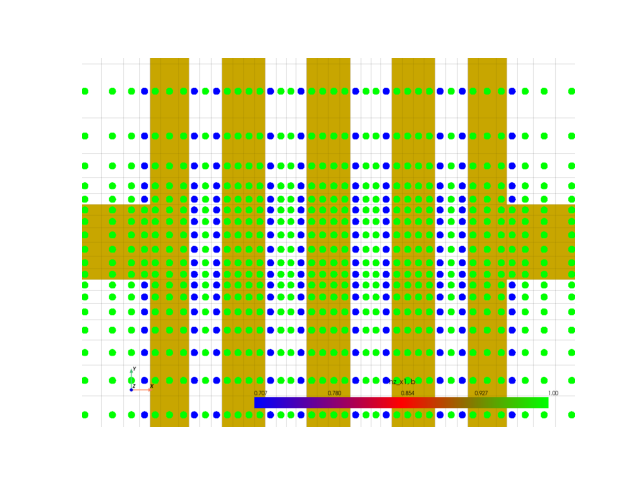
# to check the edge correction was set up properly, plot the FDTD coefficients of the H field normal to the conductor
# surface (hz in this case). The fields at the edge vary asymptotically along the x direction, so plot the hz_x1 or
# hz_x2 fields.
cpos = pv.CameraPosition(
position=(xmax/2, tap_loc, 1),
focal_point=(xmax/2, tap_loc, 0),
viewup=(0, 1, 0),
)
fig, ax = plt.subplots()
s.plot_coefficients("hz_x1", "b", "z", position=0, point_size=15, cmap="brg", camera_position = cpos, axes=ax, zoom=3)
Solve and Plot S-parameters
# create excitation pulse. Run a large number of time steps so the energy has time to either exit through the
# ports or dissipate.
pulse_n = 50000
vsrc = 1e-2 * s.gaussian_source(width=200e-12, t0=130e-12, t_len = pulse_n * s.dt)
s.assign_excitation(vsrc, 1)
s.solve(n_threads=4)
frequency = np.arange(0.5e9, 3e9, 2e6)
# downsample the time domain data before applying the DFT to speed things up
sdata = s.get_sparameters(frequency, 1, downsample=True)
S11 = sdata.sel(b=1)
S21 = sdata.sel(b=2)
# load data simulated with finer mesh to check convergence, pulse_n=150k, d_edge = 0.0025
sdata_ref = ldarray.load(dir_ / "data/combline_fine_mesh.npy")
S11_ref = sdata_ref.sel(b=1)
S21_ref = sdata_ref.sel(b=2)
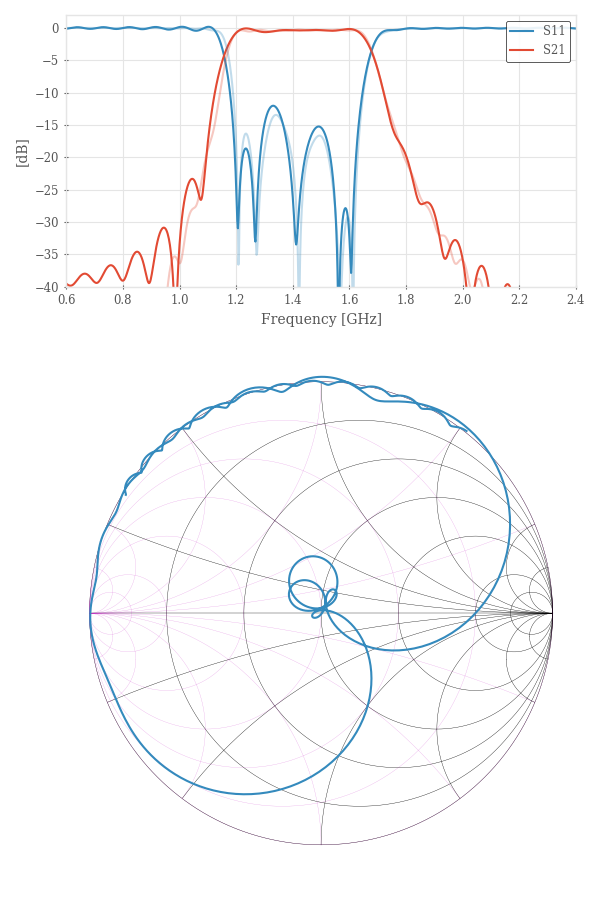
# plot smithchart and log plot
fig, (ax1, ax2) = plt.subplots(2, 1, figsize=(6, 9), height_ratios=[1, 2])
rfn.plots.draw_smithchart(ax2)
ax2.plot(S11.real, S11.imag)
ax1.plot(frequency / 1e9, rfn.conv.db20_lin(S11))
ax1.plot(frequency / 1e9, rfn.conv.db20_lin(S21))
# show finer mesh results in a lighter line style
ax1.plot(frequency / 1e9, rfn.conv.db20_lin(S11_ref), alpha=0.3, color="C0")
ax1.plot(frequency / 1e9, rfn.conv.db20_lin(S21_ref), alpha=0.3, color="C1")
ax1.set_xlabel("Frequency [GHz]")
ax1.set_xticks(np.arange(0.6, 2.6, 0.2))
ax1.set_xlim([0.6, 2.4])
ax1.set_ylabel("[dB]")
ax1.set_ylim([-40, 2])
ax1.grid(True)
ax1.legend(["S11", "S21"])
fig.tight_layout()
plt.show()
Running solver with 43.7k cells, and 50000 time steps...

Done in 19.911s
Total running time of the script: (0 minutes 20.977 seconds)