Dual-Polarized Patch Antenna

Build a dual polarized patch antenna.

Based on [1].

[1] Meltem Yildirim, “Design of Dual Polarized Wideband Microstrip Antennas”, pp. 54-70.

from pathlib import Path
import numpy as np
import matplotlib.pyplot as plt

import pyvista as pv

from np_struct import ldarray

import rfnetwork as rfn
import mpl_markers as mplm

# set matplotlib style
plt.style.use(rfn.DEFAULT_STYLE)

try:
    dir_ = Path(__file__).parent
except:
    dir_ = Path().cwd()

def phase_delay_signal(signal: ldarray, phase: float, f0: float):
    """ Apply a phase delay [radians] at f0 to time domain signal. """

    t_delay = phase / (2 * np.pi * f0)
    # number of steps that fit in the delay (rounded, no interpolation)
    dt = signal.coords["time"][1] - signal.coords["time"][0]
    n_delay = int(np.around(t_delay / dt))

    return ldarray(np.roll(signal, n_delay), coords=signal.coords)

User defined Parameters [inches]

f0 = 2.4e9
lam0 = rfn.const.c0_in / f0

# bottom substrate er
er_btm = 3.66
h_btm = 0.04
# top substrate er
er_top = 3.66
h_top = 0.06

# microstrip line width
w_ms = 0.09

# patch size
len_patch = 1.181
w_patch = 1.181

# width and length of main slot across microstrip lines
w_slot = 0.06
len_slot = 0.3

# length of cross section of slot
len_leg = 0.18

len_stub1 = 0.15
len_stub2 = 0.35

# upper slot offset (h-polarized patch)
x_pos_h = -0.37
# lower (v-polarized patch)
y_pos_v = -0.37

Build Model

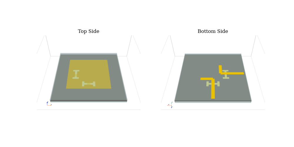
# create model
sbox = pv.Cube(center=(0, 0, 0), x_length=w_patch*2.5, y_length=w_patch*2.5, z_length=lam0 / 5)
s = rfn.FDTD_Solver(sbox)

# top substrate
sub_x0, sub_x1, sub_y0, sub_y1 = (-w_patch * 0.8, w_patch * 0.8, -len_patch * 0.8, len_patch * 0.8)
sub_top = pv.Box(bounds=(sub_x0, sub_x1, sub_y0, sub_y1, 0, h_top))
sub_btm = pv.Box(bounds=(sub_x0, sub_x1, sub_y0, sub_y1, -h_btm, 0))
s.add_dielectric(sub_top, er=er_top, style=dict(opacity=0.3))
s.add_dielectric(sub_btm, er=er_btm, style=dict(opacity=0.3))

# center ground plane layer with slot
gnd_plane = pv.Rectangle([(sub_x0, sub_y0, 0), (sub_x0, sub_y1, 0), (sub_x1, sub_y1, 0)])

#  cutout slot for side element (H)
slot_h = (x_pos_h-w_slot/2, x_pos_h+  w_slot/2, -len_slot/2, len_slot/2, 0, 0)
leg1_h = (x_pos_h-len_leg/2, x_pos_h+len_leg/2, -len_slot/2 - w_slot/2, -len_slot/2 + w_slot/2, 0, 0)
leg2_h = (x_pos_h-len_leg/2, x_pos_h+len_leg/2, len_slot/2 - w_slot/2, len_slot/2 + w_slot/2, 0, 0)

#  cutout slot for lower element (V)
slot_v = (-len_slot/2, len_slot/2, y_pos_v - w_slot/2, y_pos_v + w_slot/2, 0, 0)
leg1_v = (-len_slot/2 - w_slot/2, -len_slot/2 + w_slot/2, y_pos_v - len_leg/2, y_pos_v + len_leg/2, 0, 0)
leg2_v = (len_slot/2 - w_slot/2, len_slot/2 + w_slot/2, y_pos_v - len_leg/2, y_pos_v + len_leg/2, 0, 0)

for cutout in (slot_h, leg1_h, leg2_h, slot_v, leg1_v, leg2_v):
    gnd_plane = gnd_plane.clip_box(cutout).extract_surface(algorithm="dataset_surface")

s.add_conductor(gnd_plane, style=dict(color="grey", opacity=1))

# create patch
patch = pv.Rectangle(
    [(-w_patch/2, -len_patch/2, h_top), (-w_patch/2, len_patch/2, h_top), (w_patch/2, len_patch/2, h_top)]
)
s.add_conductor(patch, style=dict(opacity=0.6))

# microstrip feed trace for H pol slot
port_x = sub_x0 + 0.05
ms_trace_h = pv.Rectangle(
    [(port_x, -w_ms/2, -h_btm), (port_x, w_ms/2, -h_btm), (x_pos_h+len_stub1, w_ms/2, -h_btm)]
)
ms_stub_h = pv.Rectangle(
    [(x_pos_h+len_stub1 - w_ms/2, 0, -h_btm),
     (x_pos_h+len_stub1 + w_ms/2, 0, -h_btm),
     (x_pos_h+len_stub1 + w_ms/2, len_stub2, -h_btm)]
)
s.add_conductor(ms_trace_h, ms_stub_h)

# microstrip feed for V pol slot
port_y = sub_y0 + 0.05
ms_trace_v = pv.Rectangle(
    [(-w_ms/2, port_y, -h_btm), (w_ms/2, port_y, -h_btm), (w_ms/2, y_pos_v + len_stub1, -h_btm)]
)
ms_stub_v = pv.Rectangle(
    [(0, y_pos_v + len_stub1 - w_ms/2, -h_btm),
     (0, y_pos_v + len_stub1 + w_ms/2, -h_btm),
     (len_stub2, y_pos_v + len_stub1 + w_ms/2, -h_btm)]
)
s.add_conductor(ms_trace_v, ms_stub_v)

# add ports
port1_face = pv.Rectangle([(port_x, -w_ms/2, 0), (port_x, w_ms/2, 0), (port_x, w_ms/2, -h_btm)])
s.add_lumped_port(1, port1_face, "z-")

port2_face = pv.Rectangle([(-w_ms/2, port_y, 0), (w_ms/2, port_y, 0), (w_ms/2, port_y, -h_btm)])
s.add_lumped_port(2, port2_face, "z-")

# PML boundaries on all sides
s.assign_PML_boundaries("x-", "x+", "y-", "y+", "z+", "z-", n_pml=5)

# build mesh
s.generate_mesh(d_max=0.08, d_min=0.02)
# s.plot_coefficients("ex_z", "a", "z", 0).show()

# setup far-field monitor
s.add_farfield_monitor(frequency=f0)
# add near-field monitor at the plane of the slots
s.add_field_monitor("mon1", "ez", "z", 0, n_step=50)

# # show model rendering
cpos_top = pv.CameraPosition(position=(0, -3, 3), focal_point=(0, 0, 0), viewup=(0, 0.0, 1.0))
cpos_btm = pv.CameraPosition(position=(0, -3, -3), focal_point=(0, 0, 0), viewup=(0, 0.0, -1.0))

fig, (ax1, ax2) = plt.subplots(1, 2, figsize=(10, 5))
s.render(show_mesh=False, show_rulers=False, camera_position=cpos_top, axes=ax1)
s.render(show_mesh=False, show_rulers=False, camera_position=cpos_btm, axes=ax2)
ax1.set_title("Top Side")
ax2.set_title("Bottom Side")

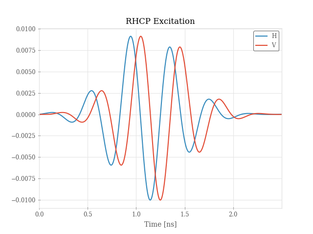
Setup RHCP excitation

# Delay the vertically polarized element excitation by 90 degrees
vsrc_h = 1e-2 * s.gaussian_modulated_source(f0, width=2000e-12, t0=1100e-12, t_len=2500e-12)
vsrc_v = phase_delay_signal(vsrc_h, phase=np.pi / 2, f0=f0)

fig, ax = plt.subplots()
ax.plot(vsrc_h.coords["time"] / 1e-9, vsrc_h)
ax.plot(vsrc_v.coords["time"] / 1e-9, vsrc_v)
ax.set_xlabel("Time [ns]")
ax.legend(["H", "V"])
ax.set_title("RHCP Excitation")

s.assign_excitation(vsrc_h, 1)
s.assign_excitation(vsrc_v, 2)

Plot Fields of RHCP excitation

s.solve(n_threads=4)

# plot near field data
gif_setup = dict(file = dir_ / "../docs/_static/img/dp_patch.gif", fps=15, step_ps=20)
s.plot_monitor("mon1", camera_position="xy", gif_setup=gif_setup)

Running solver with 184.9k cells, and 2689 time steps...

Done in 7.584s

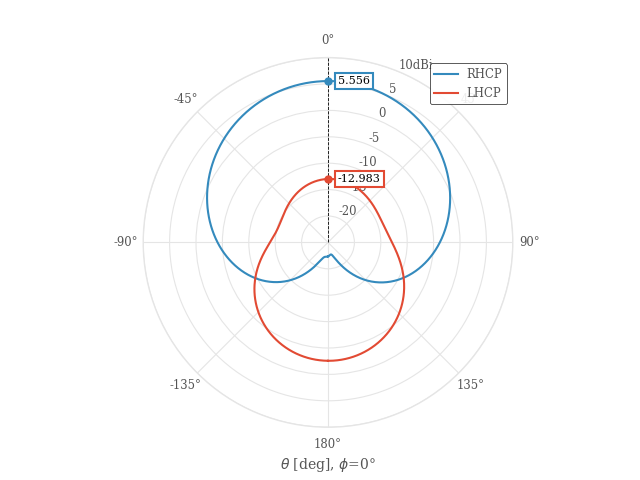
Get Far-field Patterns

# solve again with a longer time window to allow all the energy to escape the solve box.
vsrc_h_long = s.gaussian_modulated_source(f0, width=100e-12, t0=60e-12, t_len=10000e-12)
vsrc_v_long = phase_delay_signal(vsrc_h_long, phase=np.pi / 2, f0=f0)

s.reset_excitations()
s.assign_excitation(vsrc_h_long, 1)
s.assign_excitation(vsrc_v_long, 2)

s.solve(n_threads=4)

# plot far-field cut along theta at phi=0
theta_cut = rfn.conv.db10_lin(
    s.get_farfield_gain(theta=np.arange(-180, 181, 2), phi=0, polarization=["rhcp", "lhcp"])
)

theta_cut = theta_cut.interpolate(theta=np.arange(-180, 180.5, 0.5))

fig1, ax = plt.subplots(subplot_kw=dict(projection="polar"))
theta_rad = np.deg2rad(theta_cut.coords["theta"])
ax.plot(theta_rad, theta_cut.squeeze().T)

ax.set_theta_zero_location('N')
ax.set_theta_direction(-1)
ax.set_ylim([-25, 10])
ax.set_yticks(np.arange(-25, 15, 5))
ax.set_yticklabels(["", "-20", "-15", "-10", "-5", "0", "5", "10dBi"])

# Set theta labels
ax.set_xticks(np.linspace(0, 2 * np.pi, 8, endpoint=False))
labels = [f"{d}°" for d in [0, 45, 90, 135, 180, -135, -90, -45]]
ax.set_xticklabels(labels)

ax.set_xlabel(r"$\theta$ [deg], $\phi$=0°")
ax.legend(["RHCP", "LHCP"])
mplm.line_marker(x=0)

Running solver with 184.9k cells, and 10759 time steps...

Done in 29.677s

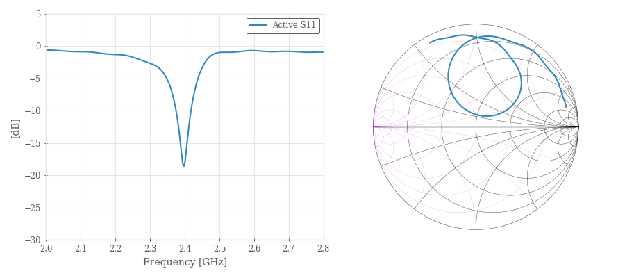
Plot S11

both port 1 and 2 are driven with an excitation, so the s-parameters plotted here are active s-parameters.

frequency: np.ndarray = np.arange(2e9, 2.802e9, 2e6)
sdata = rfn.Component_Data(s.get_sparameters(frequency))

fig, (ax1, ax2) = plt.subplots(1, 2, figsize=(9, 4))
sdata.plot(11, fmt="db", axes=ax1)
sdata.plot(11, fmt="smith", axes=ax2)
ax1.set_ylim([-30, 5])
ax1.legend(["Active S11"])
ax2.legend().remove()
fig.tight_layout()

plt.show()