Dipole Antenna

Simulate dipole antenna and plot far-field gain.

import numpy as np
import matplotlib.pyplot as plt
from rfnetwork import const, conv
import pyvista as pv

import rfnetwork as rfn
import mpl_markers as mplm

# set matplotlib style
plt.style.use(rfn.DEFAULT_STYLE)

User defined Parameters [inches]

# trace width
ms_w = 0.030

# solve box size
sbox_h = 1.2
sbox_w = 0.8
sbox_len = 0.8

# gap between dipole legs
gap = 0.015
# end to end dipole length
dipole_len = 0.546

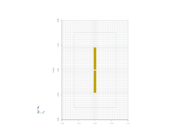
Build Dipole Model

# edges of traces along y axis
ms_y = (-ms_w / 2, ms_w / 2)

# edges of traces along z axis
ms1_z = (-(dipole_len / 2), -gap/2)
ms2_z = (gap / 2, (dipole_len / 2))

# solve box
sbox = pv.Cube(center=(0, 0, 0), x_length=sbox_len, y_length=sbox_w, z_length=sbox_h)

# upper leg of dipole
ms_upper = pv.Rectangle([
    (0, ms_y[0], ms1_z[0]),
    (0, ms_y[1], ms1_z[0]),
    (0, ms_y[1], ms1_z[1])
])

# lower leg
ms_lower = pv.Rectangle([
    (0, ms_y[0], ms2_z[0]),
    (0, ms_y[1], ms2_z[0]),
    (0, ms_y[1], ms2_z[1])
])

# port between upper and lower leg
port1_face = pv.Rectangle([
    (0, ms_y[0], gap/2),
    (0, ms_y[1], gap/2),
    (0, ms_y[1], -gap/2)
])

s = rfn.FDTD_Solver(sbox)
s.add_conductor(ms_upper, ms_lower, style=dict(color="gold"))
s.add_lumped_port(1, port1_face, "z-")

# PML boundaries are required on all sides to add a far-field monitor
s.assign_PML_boundaries("x-", "x+", "y-", "y+", "z+", "z-", n_pml=5)
s.generate_mesh(d_max = 0.02, d_min=0.01)

# setup wide-band far-field monitor
s.add_farfield_monitor(frequency=np.arange(4, 42, 2) * 1e9)
# near-field monitor
# s.add_field_monitor("e_tot", "e_total", "y", 0, n_step=10)

# apply edge singularity correction to the edges of traces, iterate over lower leg and upper leg
for i, ms_z in enumerate((ms1_z, ms2_z)):

    # left edge
    s.edge_correction(
        (0, ms_y[0], ms_z[0]),
        (0, ms_y[0], ms_z[1]),
        integration_line="y-"
    )

    # right edge
    s.edge_correction(
        (0, ms_y[1], ms_z[0]),
        (0, ms_y[1], ms_z[1]),
        integration_line="y+"
    )

    # top/lower edge
    s.edge_correction(
        (0, ms_y[0], ms_z[i]),
        (0, ms_y[1], ms_z[i]),
        integration_line=("z-" if i == 0 else "z+")
    )


cpos = pv.CameraPosition(
    position=(3, 0, 0.0),
    focal_point=(0, 0, 0),
    viewup=(0, 0.0, 1.0),
)

fig, ax = plt.subplots(1, 1)
plotter = s.render(show_mesh=True, camera_position=cpos, zoom=0.4, axes=ax)

Setup Excitation and Solve

vsrc = s.gaussian_source(width=50e-12, t0=40e-12, t_len=600e-12)
s.assign_excitation(vsrc, 1)
s.solve(n_threads=4)

Running solver with 107.5k cells, and 1291 time steps...

Done in 13.475s

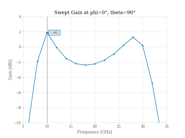
Swept Gain at phi=0°, theta=90°

ff_swept_gain = s.get_farfield_gain(theta=90, phi=[0]).sel(polarization="thetapol")

fig, ax = plt.subplots(1, 1)
ax.plot(ff_swept_gain.coords["frequency"]  / 1e9, rfn.conv.db10_lin(ff_swept_gain).squeeze(), marker=".")

ax.set_xlabel("Frequency [GHz]")
ax.set_ylabel("Gain [dBi]")
ax.set_ylim([-10, 4])
ax.set_xlim([5, 35])
ax.grid(True)
ax.set_title("Swept Gain at phi=0°, theta=90°")
mplm.line_marker(x=10)

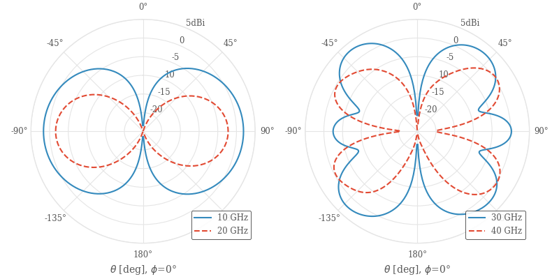
Principal Plane Cut at phi=0°

This plot shows realized gain

import time
stime = time.time()
pp_gain = rfn.conv.db10_lin(
    s.get_farfield_gain(theta=np.arange(-180, 181, 1), phi=[0]).sel(polarization="thetapol")
)
# print(time.time() - stime)

fig, (ax1, ax2) = plt.subplots(1, 2, subplot_kw=dict(projection="polar"), figsize=(8, 4))

# plot settings
line_style = ["-", "--", "-", "--"]
p_freq = [10e9, 20e9, 30e9, 40e9]
p_axes = [ax1, ax1, ax2, ax2]

theta_rad = np.deg2rad(pp_gain.coords["theta"])

for i, f in enumerate(p_freq):
    p_axes[i].plot(theta_rad, pp_gain.sel(frequency=f).squeeze(), label=f"{f/1e9:.0f} GHz", linestyle=line_style[i])

for ax in (ax1, ax2):
    ax.set_theta_zero_location('N')
    ax.set_theta_direction(-1)
    ax.set_xlabel(r"$\theta$ [deg], $\phi$=0°")
    ax.set_ylim([-25, 5])
    ax.set_yticks(np.arange(-25, 10, 5))
    ax.set_yticklabels(["", "-20", "-15", "10", "-5", "0", "5dBi"])
    ax.legend(loc="lower right")

    # Set theta labels
    ax.set_xticks(np.linspace(0, 2 * np.pi, 8, endpoint=False))
    labels = [f"{d}°" for d in [0, 45, 90, 135, 180, -135, -90, -45]]
    ax.set_xticklabels(labels)

fig.tight_layout()

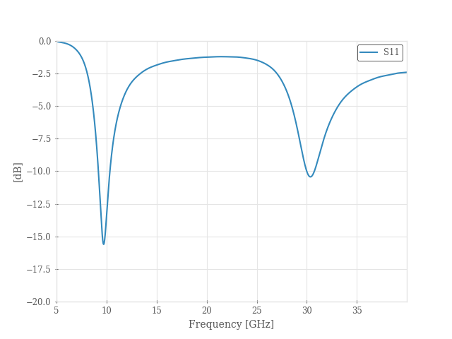
Plot S11

frequency: np.ndarray = np.arange(5e9, 40e9, 10e6)
sdata = s.get_sparameters(frequency, downsample=False)
S11 = sdata[:, 0]

fig, ax = plt.subplots()
ax.plot(frequency / 1e9, conv.db20_lin(S11))
ax.set_ylim([-20, 0])
ax.set_xlabel("Frequency [GHz]")
ax.set_ylabel("[dB]")
ax.legend(["S11"])

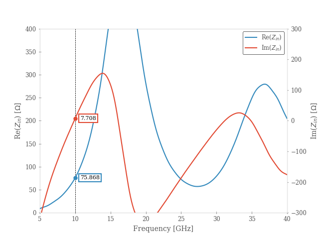
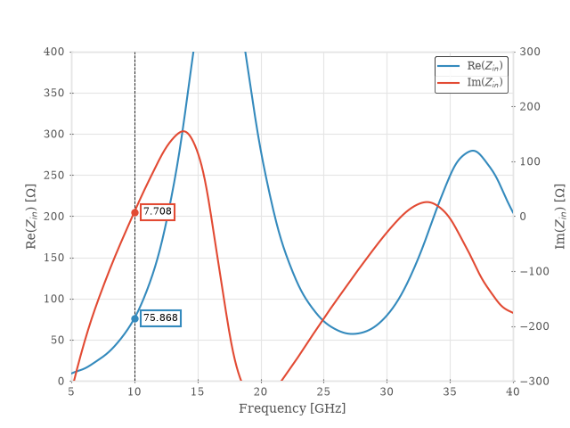
Plot Input Impedance

fig, ax = plt.subplots()
ax2 = ax.twinx()
ln1 = ax.plot(frequency / 1e9, conv.z_gamma(S11).real, label=r"Re($Z_{in}$)")
ln2 = ax2.plot(frequency / 1e9, conv.z_gamma(S11).imag, color="C1", label=r"Im($Z_{in}$)")
mplm.line_marker(x = 10, axes=ax)
ax.grid()

ax.set_xlabel("Frequency [GHz]")
ax.set_ylabel(r"Re($Z_{in}$) [$\Omega$]")
ax2.set_ylabel(r"Im($Z_{in}$) [$\Omega$]")
ax.set_ylim([0, 400])
ax.set_xlim([5, 40])
ax2.set_ylim([-300, 300])

# combined legend
handles = ln1 + ln2
labels = [h.get_label() for h in handles]
ax.legend(handles, labels, loc="upper right")

plt.show()