Microstrip Line

Simple microstrip example showing basic usage of solver.

import numpy as np
import matplotlib.pyplot as plt
from rfnetwork import const, conv, utils
import pyvista as pv

import rfnetwork as rfn
import mpl_markers as mplm

# set matplotlib style
plt.style.use(rfn.DEFAULT_STYLE)

User defined Parameters [inches]

# line width, length
ms_w = 0.04
ms_len = 1

# solve box dimensions
sbox_h = 0.4
sbox_w = 1
sbox_len = ms_len * 2

# substrate height, and dk
sub_h = 0.02
er = 3.66

Build Model

# get the expected impedance of the line
line_ref = rfn.elements.MSLine(h=sub_h, er=er, w=ms_w, length=ms_len * 1.0)
z_ref = line_ref.get_properties(10e9).sel(value="z0").item()

sbox = pv.Cube(center=(0, 0, sbox_h/2), x_length=sbox_len, y_length=sbox_w, z_length=sbox_h)
s = rfn.FDTD_Solver(sbox)

substrate = pv.Cube(center=(0, 0, sub_h/2), x_length=sbox_len, y_length=sbox_w, z_length=sub_h)
s.add_dielectric(substrate, er=er, style=dict(opacity=0.0))

ms_x = ((-ms_len/2), (ms_len/2))
ms1_y = 0

# microstrip line
ms1_trace = pv.Rectangle([
    (ms_x[0], ms1_y - ms_w/2, sub_h),
    (ms_x[0], ms1_y + ms_w/2, sub_h),
    (ms_x[1], ms1_y + ms_w/2, sub_h)
])

# port faces from line to the ground plane
port1_face = pv.Rectangle([
    (ms_x[0], ms1_y - ms_w/2, sub_h),
    (ms_x[0], ms1_y + ms_w/2, sub_h),
    (ms_x[0], ms1_y + ms_w/2, 0),
])

port2_face = pv.Rectangle([
    (ms_x[1], ms1_y - ms_w/2, sub_h),
    (ms_x[1], ms1_y + ms_w/2, sub_h),
    (ms_x[1], ms1_y + ms_w/2, 0),
])

s.add_conductor(ms1_trace, style=dict(color="gold"))
s.add_lumped_port(1, port1_face, "z+")
s.add_lumped_port(2, port2_face, "z+")

s.assign_PML_boundaries("z+", n_pml=7)

s.generate_mesh(d_max = 0.02, d_min=0.005)

# apply edge correction on either side of line
p1 = (ms_x[0], + ms_w/2, sub_h)
p2 = (ms_x[1], + ms_w/2, sub_h)
s.edge_correction(p1, p2, f"y+")

p1 = (ms_x[0], - ms_w/2, sub_h)
p2 = (ms_x[1], - ms_w/2, sub_h)
s.edge_correction(p1, p2, f"y-")

# s.plot_coefficients("ex_z", "a", "z", sub_h, point_size=15, cmap="brg", axes=ax, camera_position="xy", zoom=5)

Add Voltage and Current Monitors

# define 2D surface to measure current through
current_face = pv.Rectangle([
    (0, ms1_y - ms_w/2 - 0.001, sub_h + 0.001),
    (0, ms1_y + ms_w/2 + 0.001, sub_h + 0.001),
    (0, ms1_y + ms_w/2 + 0.001, sub_h - 0.001),
])
s.add_current_probe("c1", current_face)

# measure voltage along a 1D line from the center of the trace to ground.
voltage_line = pv.Line(
    [0, ms1_y, sub_h], [0, ms1_y, 0]
)
s.add_voltage_probe("v1", voltage_line)

Solve

vsrc = 1e-2 * s.gaussian_source(width=80e-12, t0=60e-12, t_len=500e-12)
s.assign_excitation(vsrc, 1)
s.solve(n_threads=4)

Running solver with 134.8k cells, and 2151 time steps...

Done in 3.204s

Plot Probe Values

# get the current and voltage values from each probe
line_i = s.vi_probe_values("c1")
line_v = s.vi_probe_values("v1")

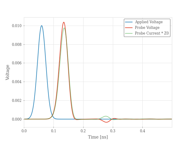
# plot time domain voltage from probe
fig, ax = plt.subplots()
ax.plot(s.time / 1e-9, vsrc, label="Applied Voltage")
ax.plot(s.time / 1e-9, line_v, label="Probe Voltage")
ax.plot(s.time / 1e-9, line_i * 50, alpha=0.5, label="Probe Current * Z0")
ax.legend()
ax.set_xlabel("Time [ns]")
ax.set_ylabel("Voltage")

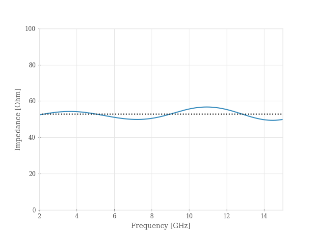
# convert probe current and voltage to frequency domain
frequency: np.ndarray = np.arange(2e9, 15e9, 10e6)
IP = utils.dtft(s.vi_probe_values("c1"), frequency, 1 / s.dt)
VP = utils.dtft(s.vi_probe_values("v1"), frequency, 1 / s.dt)
# impedance of line
ZP = VP / IP

# plot line impedance. This is a rough approximation because the H and E fields are offset
# in the grid, and we are comparing them directly without interpolation.
# The ripple is expected since the line is not perfectly matched to the load (50 ohms.)
# See tests for how to compute impedance with a PML layer that removes the reflection.
fig, ax = plt.subplots()
ax.plot(frequency / 1e9, ZP.real)
ax.set_ylim([0, 100])
ax.axhline(y=z_ref, linestyle=":", color="k")
ax.set_xlabel("Frequency [GHz]")
ax.set_ylabel("Impedance [Ohm]")

• 
• 

Plot S-parameters

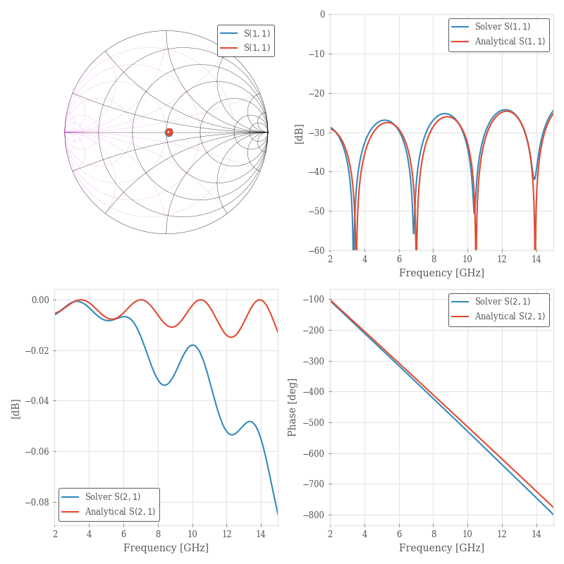
# get s-parameters
sdata = rfn.Component_Data(s.get_sparameters(frequency))

# smithchart of S11
fig, axes = plt.subplots(2, 2, figsize=(8, 8))
ax = axes[0,0]
sdata.plot(11, fmt="smith", axes=ax)
line_ref.plot(11, fmt="smith", axes=ax, frequency=frequency)

# logplot S11
ax = axes[0,1]
sdata.plot(11, fmt="db", axes=ax, label="Solver ")
line_ref.plot(11, fmt="db", axes=ax, frequency=frequency, label="Analytical ")
ax.set_ylim([-60, 0])

# logplot S21
ax = axes[1,0]
sdata.plot(21, fmt="db", axes=ax, label="Solver ")
line_ref.plot(21, fmt="db", axes=ax, frequency=frequency, label="Analytical ")
ax.legend(loc="lower left")

# phase of S21
ax = axes[1,1]
sdata.plot(21, fmt="ang_unwrap", axes=ax, label="Solver ")
line_ref.plot(21, fmt="ang_unwrap", axes=ax, frequency=frequency, label="Analytical ")

fig.tight_layout()
plt.show()