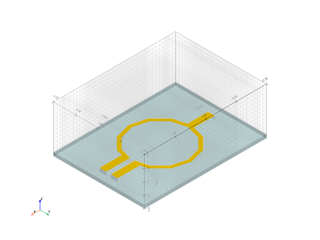
Wilkinson Combiner

Create a 3D model of a Wilkinson combiner.

import numpy as np
import matplotlib.pyplot as plt
from rfnetwork import const, conv, utils
import pyvista as pv
from np_struct import ldarray
from pathlib import Path

import rfnetwork as rfn
import mpl_markers as mplm

# set matplotlib style
plt.style.use(rfn.DEFAULT_STYLE)

try:
    dir_ = Path(__file__).parent
except:
    dir_ = Path().cwd()

Design Parameters

# values are in inches
ms_w = 0.043  # 50 ohms trace width
ms_70w = 0.023  # 70 ohm trace width
sub_h = 0.02  # substrate height
gap = 0.03  # gap between traces on port 2 and 3
er = 3.66  # relative permittivity of substrate

f0 = 3e9  # design frequency of combiner
frequency = np.arange(1e9, 5e9, 10e6)

Build Model

# y axis positions of the three port traces
ms1_y = 0
ms2_y = (gap / 2) + (ms_w / 2)
ms3_y = -(gap / 2) - (ms_w / 2)

# get quarter wavelength at the design frequency
msline70p7 = rfn.elements.MSLine(w=ms_70w, h=sub_h, er=er)
len_qw = msline70p7.get_wavelength(f0) / 4

# radius of curved section. Half the circumference should be len_qw
radius = len_qw.item() / np.pi

# Inner and outer radius are the line edges
inner_radius = radius + (ms_70w / 2)
outer_radius = radius - (ms_70w / 2)

ms_x = (-outer_radius - 0.15, -radius)
ms2_x = (radius - 0.01, outer_radius + 0.15)

# solve box dimensions
sbox_w = 2 * radius + 0.2
sbox_len = 2 * radius + 0.4
sbox_h = 0.3

# initialize model with substrate
substrate = pv.Cube(center=(0, 0, sub_h/2), x_length=sbox_len, y_length=sbox_w, z_length=sub_h)
sbox = pv.Cube(center=(0, 0, sbox_h/2), x_length=sbox_len, y_length=sbox_w, z_length=sbox_h)

s = rfn.FDTD_Solver(sbox)
s.add_dielectric(substrate, er=3.66, loss_tan=0.002, f0=f0, style=dict(opacity=0.4))

# add port 1 trace
ms1_trace = pv.Rectangle([
    (ms_x[0], ms1_y - ms_w/2, sub_h),
    (ms_x[0], ms1_y + ms_w/2, sub_h),
    (ms_x[1], ms1_y + ms_w/2, sub_h)
])
s.add_conductor(ms1_trace, style=dict(color="gold"))

port1_face = pv.Rectangle([
    (ms_x[0], ms1_y - ms_w/2, sub_h),
    (ms_x[0], ms1_y + ms_w/2, sub_h),
    (ms_x[0], ms1_y + ms_w/2, 0),
])
s.add_lumped_port(1, port1_face, "z-")

# port 2 and 3 traces, both have the same x values
for i, ms_y in enumerate((ms2_y, ms3_y)):
    ms_trace = pv.Rectangle([
        (ms2_x[0], ms_y - ms_w/2, sub_h),
        (ms2_x[0], ms_y + ms_w/2, sub_h),
        (ms2_x[1], ms_y + ms_w/2, sub_h)
    ])
    s.add_conductor(ms_trace, style=dict(color="gold"))

    port_face = pv.Rectangle([
        (ms2_x[1], ms_y - ms_w/2, sub_h),
        (ms2_x[1], ms_y + ms_w/2, sub_h),
        (ms2_x[1], ms_y + ms_w/2, 0),
    ])
    s.add_lumped_port(i+2, port_face, "z-")

# 70 ohm legs of combiner
ring = pv.Disc(
    center=(0, 0, sub_h),
    inner=inner_radius,
    outer=outer_radius,
    normal=(0, 0, 1),
    r_res=1,       # radial resolution (1 = ring)
    c_res=12       # angular resolution
)

# remove section in ring for resistor
ring = ring.clip_box((0, outer_radius + 0.1, -gap / 2, gap / 2, 0, sub_h)).extract_surface(algorithm="dataset_surface")
s.add_conductor(ring, style=dict(color="gold"))

# add 100 ohm resistor lumped element
resistor = pv.Rectangle([
    (radius - 0.01, -gap/2, sub_h),
    (radius - 0.01, gap/2, sub_h),
    (radius + 0.01, gap/2, sub_h),
])
s.add_resistor(resistor, 100, integration_line="y+")

# assign PML boundary on top face
s.assign_PML_boundaries("z+", n_pml=5)

# create mesh with a nominal width of 20mils far from geometry edges, and 5mils near edges.
s.generate_mesh(d_max=0.02, d_min=0.005)

# plot model
fig, ax = plt.subplots()
plotter = s.render(axes=ax, zoom=1)
fig.tight_layout()

# show coefficient values at the substrate
# p = s.plot_coefficients("ex_z", "a", "z", sub_h, point_size=15, cmap="brg")
# p.camera_position = "xy"
# p.show()

Run Simulation

To generate the full s-parameter matrix, each port needs to be solved individually.

# add 2D field monitor normal to the z-axis at the top of the substrate
s.add_field_monitor("mon1", "e_total", "z", position=sub_h, n_step=30)

# create excitation waveform.
vsrc = 1e-2 * s.gaussian_modulated_source(f0, width=400e-12, t0=200e-12, t_len=600e-12)


# initialize empty s-matrix data
sdata = ldarray(
    np.zeros((len(frequency), 3, 3), dtype="complex128"),
    coords=dict(frequency=frequency, b=[1, 2, 3], a=[1, 2, 3])
)

# solve each of the 3 ports
for port in range(1, 4):
    print(f"Solving Port {port}")
    s.reset_excitations()
    s.assign_excitation(vsrc, port)
    s.solve()

    # populate the column of the s-matrix with this port as the input wave
    sdata[dict(a=port)] = s.get_sparameters(frequency, source_port=port, downsample=False).sel(a=port)


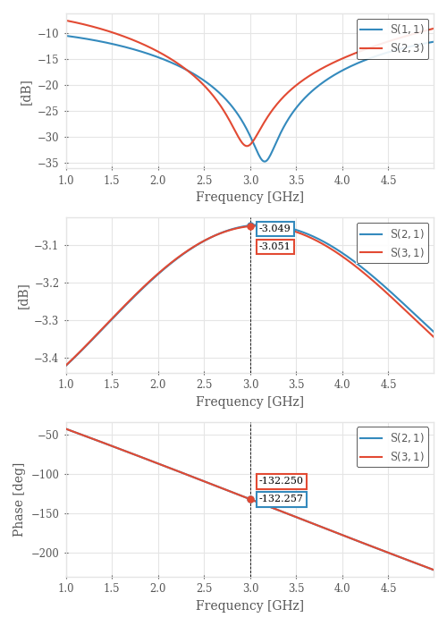
# plot s-parameter results
wilk = rfn.Component_Data(sdata)
fig, (ax1, ax2, ax3) = plt.subplots(3, 1, figsize=(5, 7))
wilk.plot(11, 23, axes=ax1)
wilk.plot(21, 31, axes=ax2)
wilk.plot(21, 31, fmt="ang_unwrap", axes=ax3)
mplm.line_marker(x=f0/1e9, axes=ax2)
mplm.line_marker(x=f0/1e9, axes=ax3)
fig.tight_layout()
plt.show()

Solving Port 1
Running solver with 159.4k cells, and 2753 time steps...

Done in 4.596s
Solving Port 2
Running solver with 159.4k cells, and 2753 time steps...

Done in 4.594s
Solving Port 3
Running solver with 159.4k cells, and 2753 time steps...

Done in 4.604s

Visualize Fields

Plot the total electric field from the filed monitor when used as a combiner with equal signals on port 2 and 3.

s.reset_excitations()
s.assign_excitation(vsrc, 2)
s.assign_excitation(vsrc, 3)
s.solve()

# To generate the full s-parameter matrix, each port needs to be solved individually.
gif_setup = dict(file = dir_ / "../docs/_static/img/wilkinson.gif", fps=15, step_ps=5)
p = s.plot_monitor(["mon1"], camera_position="xy", vmax=30, vmin=0, gif_setup=gif_setup)

Running solver with 159.4k cells, and 2753 time steps...

Done in 4.601s