Filters

Examples of basic, lumped element filter.

import rfnetwork as rfn
import numpy as np
import matplotlib.pyplot as plt

# set matplotlib style
plt.style.use(rfn.DEFAULT_STYLE)

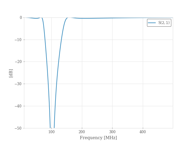
Bandstop Filter

bsf = rfn.elements.LumpedElementFilter.from_chebyshev(fc=(70e6, 150e6), btype="bandstop", n=3)

frequency = np.arange(10e6, 0.5e9, 1e6)

fig, ax = plt.subplots()
bsf.plot(21, freq_unit="mhz", frequency=frequency, axes=ax)
ax.set_ylim([-50, 0]);

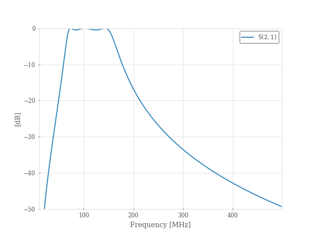
Bandpass Filter

bpf = rfn.elements.LumpedElementFilter.from_chebyshev(fc=(70e6, 150e6), btype="bandpass", n=3)

frequency = np.arange(10e6, 0.5e9, 1e6)

fig, ax = plt.subplots()
bpf.plot(21, freq_unit="mhz", frequency=frequency, axes=ax)
ax.set_ylim([-50, 0]);

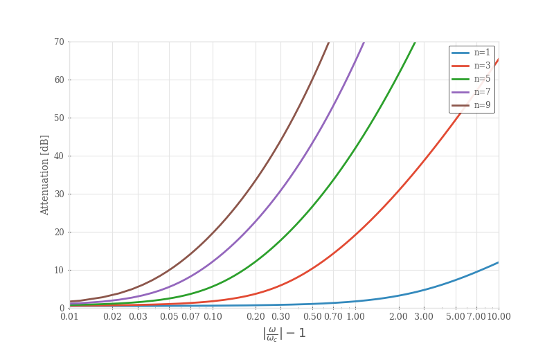
Lowpass Filter

Generate Figures 8.27a (0.5 Ripple) in Pozar 4th ed.

fc = 150e6
frequency = np.logspace(0, 11, 5000)
n_list = [1, 3, 5, 7, 9]

fig, ax = plt.subplots(1, 1, figsize=(8, 5))

for n in n_list:
    # build lowpass filter network
    lpf = rfn.elements.LumpedElementFilter.from_chebyshev(fc, btype="lowpass", n=n)
    sdata = lpf.evaluate(frequency)["s"]
    ax.plot((frequency / fc) - 1, -rfn.conv.db20_lin(sdata.sel(b=2, a=1)), linewidth=2)

# plot formatting
ax.set_ylim([0, 70])
ax.set_xscale("log")
ax.set_xlim([10e-2, 10])
ax.grid(True)
base_xticks = np.array([1, 2, 3, 5, 7])
xticks = np.concatenate([base_xticks * 1e-2, base_xticks * 1e-1, base_xticks, [10]])
ax.set_xticks(xticks)
ax.set_xticklabels([f"{x:.2f}" for x in xticks], fontsize=9)

ax.legend([f"n={n}" for n in n_list])
ax.set_xlabel(r"$|\frac{\omega}{\omega_c}| - 1$", fontsize=13)
ax.set_ylabel("Attenuation [dB]")

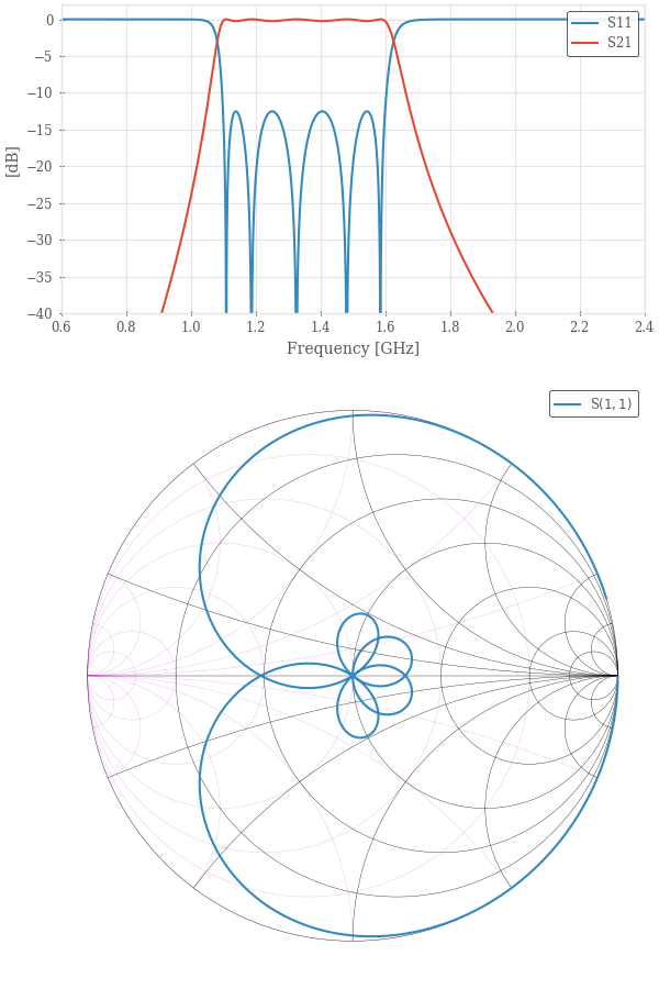
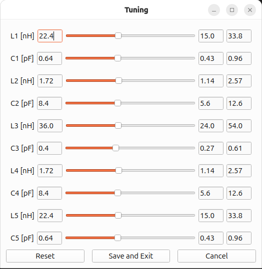
Filter Tuning

Interactively tune a lumped element band-pass filter.

# This uses the same prototype values as the combline_stripline example. The tuning parameters can give a sense
# for how the elements of the real filter affect the filter response.

f1 = 1.1e9
f2 = 1.6e9

g = rfn.utils.chebyshev_prototype(5, 0.25)
print(g)

bpf = rfn.elements.LumpedElementFilter(fc=(f1, f2), btype="bandpass", prototype=g)

frequency = np.arange(10e6, 3e9, 1e6)

fig, (ax1, ax2) = plt.subplots(2, 1, figsize=(6, 9), height_ratios=[1, 2], constrained_layout=True)
bpf.plot(11, 21, freq_unit="ghz", frequency=frequency, axes=ax1, tune=True)
ax1.set_ylim([-30, 2])

bpf.plot(11, freq_unit="ghz", fmt="smith", frequency=frequency, axes=ax2, tune=True)

ax1.set_xlabel("Frequency [GHz]")
ax1.set_xticks(np.arange(0.6, 2.6, 0.2))
ax1.set_xlim([0.6, 2.4])
ax1.set_ylabel("[dB]")
ax1.set_ylim([-40, 2])
ax1.grid(True)
ax1.legend(["S11", "S21"])

tuners = [
    dict(component="S1.l1", label="L1 [nH]", multiplier=1e-9),
    dict(component="S1.c2", label="C1 [pF]", multiplier=1e-12),
    dict(component="P2.l1", label="L2 [nH]", multiplier=1e-9),
    dict(component="P2.c2", label="C2 [pF]", multiplier=1e-12),
    dict(component="S3.l1", label="L3 [nH]", multiplier=1e-9),
    dict(component="S3.c2", label="C3 [pF]", multiplier=1e-12),
    dict(component="P4.l1", label="L4 [nH]", multiplier=1e-9),
    dict(component="P4.c2", label="C4 [pF]", multiplier=1e-12),
    dict(component="S5.l1", label="L5 [nH]", multiplier=1e-9),
    dict(component="S5.c2", label="C5 [pF]", multiplier=1e-12),
]

# start the tuner (turned off for the readthedocs runner)
# bpf.tune(tuners)

[1.0, 1.414460379957097, 1.3179959561391665, 2.241408252195952, 1.3179959561391663, 1.4144603799570974, 1.0]

# print tuned values (unless tune was canceled, then this just shows the initial values)
bpf.print_state()

S1:
   l1: (value: 22.512e-9)
   c2: (value: 639.318e-15)
P2:
   l1: (value: 1.715e-9)
   c2: (value: 8.391e-12)
S3:
   l1: (value: 35.673e-9)
   c2: (value: 403.447e-15)
P4:
   l1: (value: 1.715e-9)
   c2: (value: 8.391e-12)
S5:
   l1: (value: 22.512e-9)
   c2: (value: 639.318e-15)