Vivaldi Antenna

Import Gerber files of a vivaldi antenna and compare the S-parameters with measured results.

import numpy as np
import matplotlib.pyplot as plt
from rfnetwork import conv
import pyvista as pv
import rfnetwork as rfn

from pathlib import Path
import numpy as np

# set matplotlib style
plt.style.use(rfn.DEFAULT_STYLE)

try:
    dir_ = Path(__file__).parent
except:
    dir_ = Path().cwd()

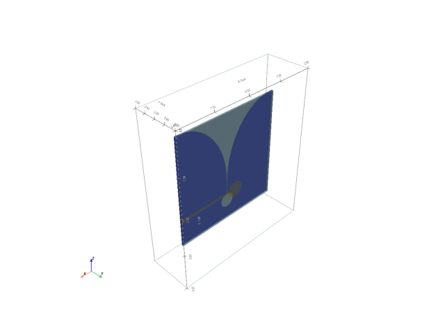
Build model

Import Gerber files into model.

# create model instance with a bounding box extending past the board files a bit to allow for PML layers.
# Boards will be placed in the xz plane.
bounding_box = pv.Box((-2.6, 2.6, -0.8, 0.8, -0.8, 4.8))
s = rfn.FDTD_Solver(bounding_box)

# add FR-4 board
sub_h = 0.06
substrate = pv.Box((-2.0, 2.0, -sub_h, 0 , 0, 4))
s.add_dielectric(substrate, er=4.5, loss_tan=0.015, f0=1e9, style=dict(opacity=0.8))

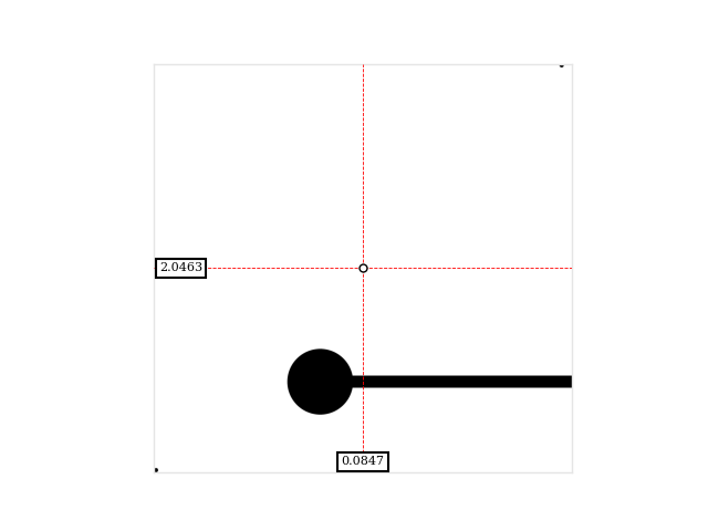
# Aligning the gerber files can be tricky since they often contain margins that go past the physical extent of the board
# The images can be plotted with interactive markers showing the physical coordinates, and allows experimenting
# with different origins.
rfn.utils_mesh.plot_gerber(dir_ / "data/lab_project-F_Cu.gbr", origin=(-1.83, 0.175))

# import bottom layer gerber file. Origin is the location of the lower left corner in the physical grid.
# this gerber file has a 20mil margin, board is placed so the corner of the usable board is at x=-2in, z=0in.
s.add_image_layer(
    filepath = dir_ / "data/lab_project-B_Cu.gbr",
    origin = (-2.0197, -sub_h, -0.0197),
    width_axis = "x",
    length_axis = "z",
    style=dict(color="blue")
)

s.add_image_layer(
    filepath = dir_ / "data/lab_project-F_Cu.gbr",
    origin = (-1.83, 0, 0.175),
    width_axis = "x",
    length_axis = "z",
    style=dict(color="gold")
)

# ensure the microstrip trace extends all the way to the edge of the board.
port_x = 2
port_y0, port_y1 = (0.949, 1.059)

trace_extension = pv.Rectangle(((port_x - 0.1, 0, port_y0), (port_x, 0, port_y0), (port_x, 0, port_y1)))
s.add_conductor(trace_extension, style=dict(color="gold"))

# add lumped port
port_face = pv.Rectangle(((port_x, -sub_h, port_y0), (port_x, -sub_h, port_y1), (port_x, 0, port_y1)))
s.add_lumped_port(1, port_face, "y+")

# Assign PML layers on all sides, including the bottom
s.assign_PML_boundaries("x-", "x+", "y-", "y+", "z+", "z-", n_pml=5)
s.generate_mesh(0.06, 0.01)

fig, ax = plt.subplots()
p = s.render(show_mesh=False, axes=ax)
p.close()

• 
• 

Setup Solver

Add field monitors/excitations and run solver

s.add_field_monitor("mon1", "e_total", axis="y", position=-sub_h, n_step=20)
s.add_farfield_monitor([2e9, 3e9])

vsrc = s.gaussian_source(width=100e-12, t0=50e-12, t_len=5000e-12)

s.assign_excitation(vsrc, 1)
s.solve()

Running solver with 384.9k cells, and 10963 time steps...

Done in 66.701s

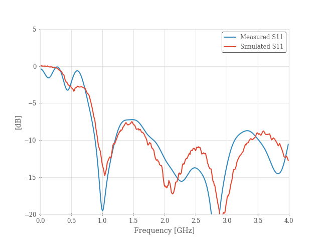
Post Processing

# get measured s-parameter data as a reference
ref_sdata = rfn.Component_SnP(dir_ / "data/vivaldi_measured.s2p")

# plot s-parameters. The grid here is quite coarse and results can be improved by lowering d_edge in generate_mesh
frequency = np.arange(0.01, 4, 0.01) * 1e9
sdata = s.get_sparameters(frequency, downsample=False)
S11 = sdata.sel(b=1)

fig, ax = plt.subplots()
ax.plot(frequency / 1e9, conv.db20_lin(S11))
ref_sdata.plot(11, frequency=frequency, axes=ax)
ax.set_ylim([-20, 5])
ax.set_xlabel("Frequency [GHz]")
ax.set_ylabel("[dB]")
ax.legend(["Measured S11", "Simulated S11"])
ax.set_xticks(np.arange(0, 4.5, 0.5))

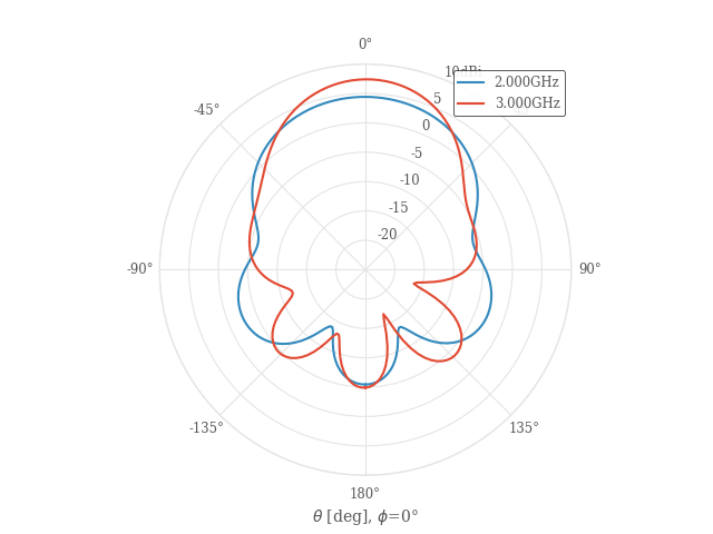
# plot far-field cut along theta at phi=0
theta_cut = rfn.conv.db10_lin(
    s.get_farfield_gain(theta=np.arange(-180, 181, 2), phi=0).sel(polarization="thetapol")
)

fig1, ax = plt.subplots(subplot_kw=dict(projection="polar"))
theta_rad = np.deg2rad(theta_cut.coords["theta"])
ax.plot(theta_rad, theta_cut.squeeze().T)

ax.set_theta_zero_location('N')
ax.set_theta_direction(-1)
ax.set_ylim([-25, 10])
ax.set_yticks(np.arange(-25, 15, 5))
ax.set_yticklabels(["", "-20", "-15", "-10", "-5", "0", "5", "10dBi"])

# Set theta labels
ax.set_xticks(np.linspace(0, 2 * np.pi, 8, endpoint=False))
labels = [f"{d}°" for d in [0, 45, 90, 135, 180, -135, -90, -45]]
ax.set_xticklabels(labels)

ax.set_xlabel(r"$\theta$ [deg], $\phi$=0°")
ax.legend(["{:.3f}GHz".format(f/1e9) for f in theta_cut.coords["frequency"]])
plt.show()

• 
• 

Plot near-field

Re-solve with a narrow-band excitation and plot near-field monitor

# excitation centered around 3 GHz. The signal still has significant broad-band energy outside of 3GHz, but it
# makes it easier to see the general response at a single frequency.
vsrc = s.gaussian_modulated_source(3e9, width=1300e-12, t0=600e-12, t_len=2000e-12)
s.reset_excitations()
s.assign_excitation(vsrc, 1)
# start solver with the new excitation
s.solve()

# plot near-field monitor and save as a .gif file
gif_setup = dict(file = dir_ / "../docs/_static/img/vivaldi.gif", step_ps=12)
p = s.plot_monitor(
    "mon1", opacity="linear", camera_position="xz", vmin=20, vmax=60, gif_setup=gif_setup
)
# p.show()

Running solver with 384.9k cells, and 4385 time steps...

Done in 29.456s