Coupled Stripline

Analyze even and odd mode impedance of coupled strip lines.

import numpy as np
import matplotlib.pyplot as plt
from rfnetwork import conv
import pyvista as pv
import rfnetwork as rfn
import mpl_markers as mplm

# set matplotlib style
plt.style.use(rfn.DEFAULT_STYLE)

Design Parameters

sl_w = 0.022  # trace width
sl_sp = 0.013  # trace spacing
b = 0.06  # substrate height
er =  3.66  # relative permittivity

# solve box dimensions, inches
sbox_h = b
sbox_w = 0.6
sbox_len = 0.25

# center locations of microstrip lines along y axis
line1_y = -(sl_w / 2) - (sl_sp / 2)
line2_y = (sl_w / 2) + (sl_sp / 2)

# end locations of lines along x axis, lines terminate in PML region
ms_x = (-sbox_len/2 + 0.1, sbox_len/2)

frequency = np.arange(5e9, 15e9, 10e6)

Create 3D Model

# substrate geometry
substrate = pv.Cube(
    center=(0, 0, 0), x_length=sbox_len, y_length=sbox_w, z_length=b
)

# solve box
sbox = pv.Cube(
    center=(0, 0, 0), x_length=sbox_len, y_length=sbox_w, z_length=b
)

s = rfn.FDTD_Solver(sbox)
s.add_dielectric(substrate, er=er, style=dict(opacity=0.0))

# add lines
for i, y in enumerate((line1_y, line2_y)):
    ms_trace = pv.Rectangle([
        (ms_x[0], y - sl_w/2, 0),
        (ms_x[0], y + sl_w/2, 0),
        (ms_x[1], y + sl_w/2, 0)
    ])
    s.add_conductor(ms_trace, style=dict(color="gold"))

    # add lumped ports
    port_face = pv.Rectangle([
        (ms_x[0], y - sl_w/2, -b/2),
        (ms_x[0], y + sl_w/2, -b/2),
        (ms_x[0], y + sl_w/2, b/2),
    ])

    integration_line = pv.Line((ms_x[0], y, -b/2), (ms_x[0], y, 0))
    s.add_lumped_port(i + 1, port_face, integration_line=integration_line)

# assign PML layers, omitting the x- side near the ports
s.assign_PML_boundaries("x+", n_pml=5)

# create mesh with a nominal width of 20mils far from geometry edges, and 2.5mils near edges.
# cell widths are tapered to minimize errors
s.generate_mesh(d_max = 0.01, d_min = 0.0025)

# apply edge singularity correction to the edges along the length of the microstrip lines
for i, y in enumerate((line1_y, line1_y)):
    p1 = (ms_x[0], y + sl_w/2, 0)
    p2 = (ms_x[1], y + sl_w/2, 0)

    s.edge_correction(p1, p2, integration_line="y+")

    p1 = (ms_x[0], y - sl_w/2, 0)
    p2 = (ms_x[1], y - sl_w/2, 0)

    s.edge_correction(p1, p2, integration_line="y-")

# add 2D field monitor normal to the x-axis at the center of the grid
s.add_field_monitor("mon1", "e_total", axis="x", position=0, n_step=10)

Setup Excitations

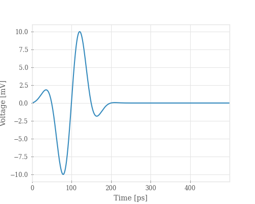
# create voltage waveform. Time units are in seconds
vsrc = 1e-2 * s.gaussian_modulated_source(f0=10e9, width=200e-12, t0=100e-12, t_len=500e-12)

fig, ax = plt.subplots(figsize=(5, 4))
ax.plot(vsrc.coords["time"] * 1e12, vsrc * 1e3)
ax.set_xlabel("Time [ps]")
ax.set_ylabel("Voltage [mV]")

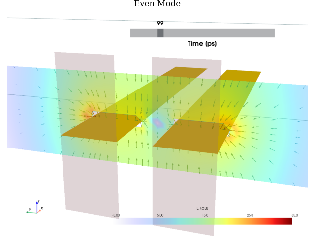
Solve Even Mode

# set up camera to view the fields near the ports, looking down the x axis
cpos = pv.CameraPosition(
    position=(-0.15, -0.05, 0.05),
    focal_point=(0, 0, 0.00),
    viewup=(0, 0.0, 1.0),
)

# arguments for plot_monitor
plot_mon_kwargs = dict(
    monitor=["mon1", "mon1"],
    style=["vectors", "surface"],  # plot both vector field and magnitude colormap
    max_vector_len=0.005,  # keep vectors shorter than 5mils
    opacity="linear",   # fade smaller field components
    init_time=100,  # start at 100ps
    show_mesh=False,
    show_rulers=False,
    camera_position=cpos,
    vmax=35,  # maximum colormap value, in dB
)

# run even mode, same waveform at both port 1 and 2
s.assign_excitation(vsrc, [1, 2])
s.solve(n_threads=4, show_progress=False)

S_even = s.get_sparameters(frequency)

fig, (ax1) = plt.subplots()
ax1.set_title("Even Mode")
s.plot_monitor(**plot_mon_kwargs, axes=ax1)

fig.tight_layout(pad=0)

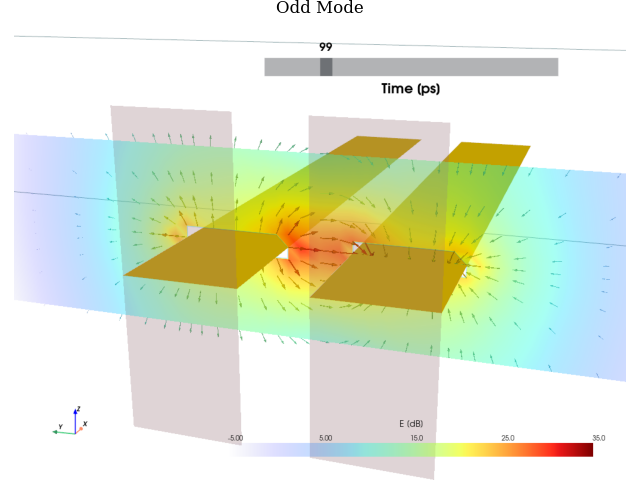
Solve Odd Mode

# setup opposite polarity waveforms at each port
s.reset_excitations()
s.assign_excitation(vsrc, 1)
s.assign_excitation(-vsrc, 2)
s.solve(n_threads=4, show_progress=False)
S_odd = s.get_sparameters(frequency)

fig, (ax2) = plt.subplots()
ax2.set_title("Odd Mode")
s.plot_monitor(**plot_mon_kwargs, axes=ax2)

fig.tight_layout(pad=0)

Coupled Line Impedance

# Compare even and odd impedance with this online solver:
# https://wcalc.sourceforge.net/cgi-bin/coupled_stripline.cgi
# ref_even_z = 72.5
# ref_odd_z = 48.2

Zo, Ze = rfn.utils.coupled_sline_impedance(sl_w, sl_sp, b, er)
print(f"Even: {Ze:.2f}, Odd: {Zo:.2f}")

fig, ax = plt.subplots()
ax.plot(frequency / 1e9, conv.z_gamma(S_odd.sel(b=1)).real)
ax.plot(frequency / 1e9, conv.z_gamma(S_even.sel(b=1)).real)

ax.set_ylim([0, 110])
ax.axhline(y=Zo, linestyle=":", color="C0")
ax.axhline(y=Ze, linestyle=":", color="C1")
ax.set_xlabel("Frequency [GHz]")
ax.set_ylabel("Impedance [Ohm]")
ax.legend(["Odd Mode", "Even Mode", "Ref Odd", "Ref Even"])
mplm.line_marker(x = 10, axes=ax)
ax.set_title("Odd/Even Impedance of Coupled Stripline")

plt.show()

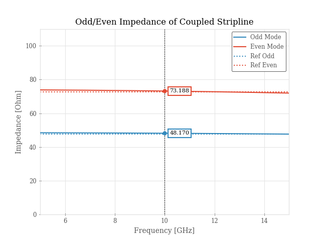
Even: 72.71, Odd: 47.71